The process of ensuring the dependability of analytical methods is known as analytical method validation. This systematic and comprehensive evaluation is indispensable for confirming that an analytical procedure consistently produces reliable and consistent results, thus bolstering the credibility of scientific findings.
Performance characteristics are crucial to the process of analytical method validation, as they serve as a comprehensive collection of criteria that are carefully assessed to determine the effectiveness of the method. These factors function as an objective standard to evaluate the suitability of the approach, guaranteeing that it not only fulfils but surpasses the rigorous, stringent standards required in various industries.
Typical Performance Characteristics for Analytical Method Validation
According to the ICH Q2(R1) guideline on Validation of Analytical Procedures and its drafted revision ICH Q2(R2), a validation study is designed to provide sufficient evidence for a certain analytical method to meet its objectives. Depending on the analytical method, these objectives can be characterized with:
- Specificity/Selectivity
- Linearity
- Range
- Accuracy
- Precision
- Detection Limit
- Quantitation Limit
- Robustness
Linearity
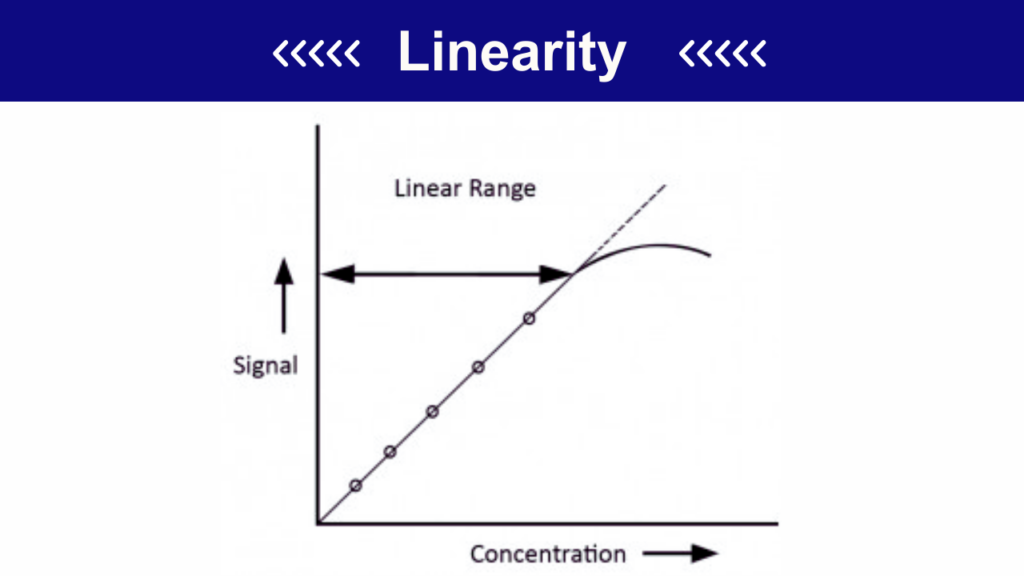
Linearity represents the capacity of an Assay to demonstrate that the method is capable of providing a direct and proportionate response to variations in analyte concentration within the working range. Depending on how samples are prepared and which analytical procedure is selected, the reportable range will correspond to a specific working range.
In order to confirm the suitability of the selected method for its intended use, it is important to demonstrate the linear relationship between analyte concentration and response across the selected working range of the method. Results are usually evaluated using appropriate statistical methods (e.g., calculating regression line by the method of least squares), in order to provide a mathematical estimation for the linearity of the method.
A minimum of five concentration points that are appropriately distributed across the entire range are recommended, but more complex methods may require additional points in order to demonstrate the linearity of the method. The acceptance criteria for the linear regression in most of the test methods will often require to be R2 > 0.95.
In certain situations, methods can show non-linear responses, but this doesn’t mean that a method can not be validated for its purpose. The suitability of the method in such cases is often assessed with a different approach by using non-linear analysis (e.g., coefficient of determination).
By demonstrating linearity, we are able to confirm the ability of an analytical method to obtain signals which are directly proportional to the concentration of the analyte in the sample. Practically, to a certain degree, it can be concluded that every time Assay samples are introduced to the method, the detection response of the method will always be proportional to analyte concentrations ranging from 80% to 120% of the specification limit.
When selecting a method for validation, we can decide whether to demonstrate Linearity by the response of the drug substance (e.g., appropriate dilutions of standard stock solution) or by separately prepared synthetic mixtures (drug substance + drug product excipients) using the proposed method.
Many times in LC-MS (Liquid Chromatography Mass Spectroscopy) for example, synthetic sample mixtures are being prepared in order to account for the possible matrix influence on the ionization of the analyte.
Range
The specific range is usually derived from linearity studies since it depends on the intended application of the procedure. With this parameter, it is established that the method will provide acceptable linearity, accuracy, and precision within the specified range.
Method Dependent Acceptable Ranges
Depending on the testing method, the acceptable range can be different:
- For drug substance and drug product Assay: 80 to 120% of the test concentration
- For Content Uniformity Assay: 70 to 130% of test concentration
- For Dissolution Test: ± 20% over the entire specification range (e.g., if the specification for a certain product with controlled-release covers a region of 20% after 1 hour, up to 80% after 24 hours, the validation range would be 0 – 110% of the labelled claim)
- For impurity Assays: From reporting level (Quantitation Limit) to 120% of the impurity specification
- For impurities known to be unusually potent or to produce toxic or unexpected pharmacological effects, the detection/Quantitation Limit should be commensurate with the level at which the impurities must be controlled.
- In analytical methods where Assay and Purity tests are performed together as one test and only a standard at 100% concentration is used, linearity should be covered from the reporting threshold (Quantitation Limit) of the impurities to 120% of labelled content for the assay.
Accuracy and Precision
Before we move on to classic definitions of accuracy and precision and how they are established, here below is a classic example for a better understanding of these two terms:
- In an imagined dartboard, the centre (bulls-eye) represents the true value of the measurement. Every dart that lands on the dartboard represents a single measurement result generated by the method.
- The closer the darts are landing to the centre, the more accurate the result is.
When darts are landing relatively close to one another in a specific area, but that area is far from the centre of the dartboard, it can be concluded that the method is very precise but, unfortunately, not accurate.
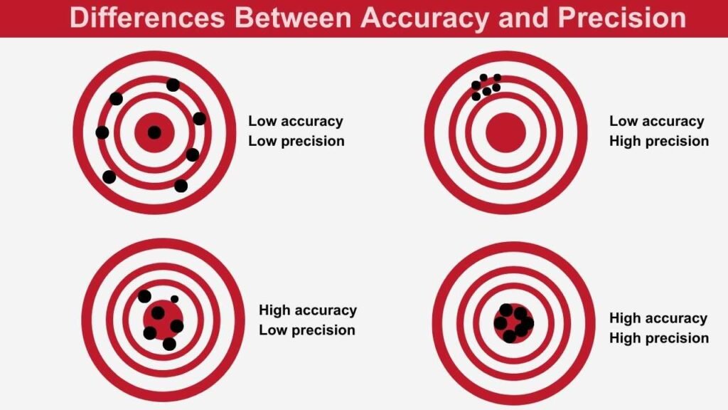
When a method is accurate and precise, it is expected for the darts (results) to land very close to one another (obtained results are with very close values), and all of them should be centered on the dartboard (experimentally obtained values are very close to theoretical values).
Accuracy
Accuracy is defined as the closeness of the test results obtained by the method to the true value. It is usually reported as the recovery (%) of the known amount or as the difference between the mean assay result and the accepted true value together with the confidence intervals.
Accuracy should be verified over the reportable range of an analytical method by comparing measured findings to their predicted values. These tests are typically demonstrated under regular testing conditions by using a true sample matrix, using the described procedure for the preparation of samples, etc.
Demonstration of Accuracy in Test Assays for Drug Substances
- Accuracy is usually demonstrated by using an analyte of known purity (a reference material or a well-characterized impurity/related substance) to obtain measurements that are later used to express and compare the experimental concentration against the theoretical concentration.
- Another way to demonstrate accuracy is when the findings of the suggested analytical technique are compared to those of a second, well-defined procedure (an orthogonal procedure) that ideally uses a distinct measuring approach. The accuracy of the second procedure should also be mentioned.
- Accuracy may be inferred once precision, linearity, and specificity have been established.
Demonstration of Accuracy in Test Assays for Drug Products
- In order to demonstrate accuracy, a known quantity of the analyte of interest is introduced to a synthetic matrix (spiked) containing all components except for the analyte of interest, and then the analytical procedure is applied.
- In situations when it is difficult to recreate all anticipated components of the drug product, known amounts of the analyte may be added to the test sample. The outcomes of both unspiked and spiked sample readings are then evaluated. Another way to demonstrate accuracy in this situation is by comparing obtained results with results from another well-characterized procedure with stated accuracy.
- Accuracy may be inferred once precision, linearity, and specificity have been established.
Demonstration of Accuracy in Impurity Quantitation Tests
- Accuracy should be assessed on samples (drug substance/drug product) that are spiked with known amounts of impurities.
- In cases when it is impossible to obtain samples of certain impurities and/or degradation products, it is considered acceptable to compare the results obtained by an independent procedure. The response factor of the drug substance can also be used. In these types of results, it is important to clearly note how individual and total impurities are calculated (e.g., weight/weight or area percentage in all cases with respect to the major analyte).
Accuracy should be assessed by using at least 3 concentration points covering the reportable range with 3 replicates for each point. For every replicate, the complete analytical procedure should be followed.
Precision
Precision represents the closeness of agreement (degree of scatter) between a series of measurements obtained from multiple sampling of the same homogeneous sample under the prescribed conditions. It may be considered at 3 levels:
Repeatability
Repeatability is used to express the precision under the same operating conditions over a short interval of time. For assessing repeatability, a minimum of 9 determinations (3 concentrations x 3 replicates) covering the reportable range or a minimum of 6 determinations at 100% of the test concentration are required
Intermediate precision (also known as Ruggedness)
Intermediate precision is used to express variations that might occur within the laboratory where tests take place. The extent to which intermediate precision should be established depends on the circumstances under which the procedure is intended to be used. Studies usually include tests performed on different days, tests performed by different analysts, tests performed on different equipment, different environmental conditions, etc.
The objective of intermediate precision validation is to verify that in the same laboratory, a method will provide the same results once the development phase is over.
Reproducibility
Reproducibility shows the ability of the method to reproduce data within the predefined precision between different labs. These data are not usually part of the marketing authorization dossier. However, when it comes to standardization of analytical procedures, such as the inclusion of procedures in pharmacopoeias, reproducibility plays a big role in establishing precision between collaborative laboratories.
Each type of precision being investigated should generally be expressed in terms of standard deviation, relative standard deviation (coefficient of variation), and confidence interval.
Validation of lower range limits (Quantitation Limit and Detection Limit)
Detection Limit (DL) is described as the lowest amount of analyte in a sample that can be detected with the method but not necessarily quantified.
Quantitation Limit (QL) is the lowest amount of analyte in a sample that can be quantified with acceptable accuracy and precision.
Estimating lower ranges
Lower range limits can be estimated using different approaches and techniques:
Based on the signal-to-noise (S/N)
This approach is suitable for analytical methods with a baseline possibility. Signal to noise, as the name implies, can be determined by obtaining values for signal and noise in the selected method. A signal is calculated by comparing the measured response of an analyte from a sample with a known low concentration against a blank sample.
The signal value, for example, in chromatographic procedures, should be determined from a defined region in the blank sample chromatogram, equally around the place where the peak of the analyte would be found. Sometimes an appropriate and representative baseline region can also be used instead of running blank samples.
DL and QL are starting concentrations of the method where the analyte can be reliably detected or quantified, respectively. A signal-to-noise ratio of 3:1 is usually considered acceptable in order to estimate the concentration at which an analyte can be detected, whereas a signal-to-noise ratio of at least 10:1 is considered acceptable as the lowest concentration point at which a method is capable of reliably quantifying the analyte.
Based on the Standard Deviation of a Linear Response and a Slope
The Detection Limit (DL) can be expressed as:
DL=(3*σ)/S
The Quantitation Limit (QL) can be expressed as:
QL=(10*σ)/S
where,
σ = the standard deviation of the response; S = the slope of the calibration curve;
The slope S can be determined from the regression line of the analyte.
The estimate of the standard deviation of the response (σ) can be carried out in three ways, based on:
- Standard Deviation of the Blank (measuring background responses on an appropriate number of blank samples, then calculating their standard deviation)
- Calibration Curve (A specific calibration curve should be evaluated using samples containing an analyte in the range of the DL and QL. The residual standard deviation (root mean square error/deviation) of the regression line or the standard deviation of y-intercepts of the regression line can be used as the standard deviation.)
- Visual evaluation (may be used for both non-instrumental and instrumental methods)
Based on Accuracy and Precision at lower range limits
Instead of using estimated values, QL can be directly validated by accuracy and precision measurements.
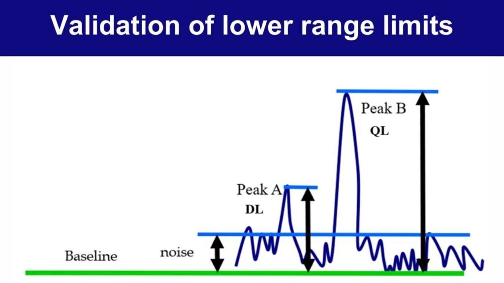
According to the presented image, it can be noted that Peak A represents the Detection Limit response which is approximately 3 times the height of the noise interval, while Peak B, representing the Quantitation Limit, is approximately 10 times the height of the noise interval (note DL/QL formulas presented above). This means that if any acquired peak is “smaller” than Peak A, the method wouldn’t be capable of differentiating whether this action peak is an analyte response or just a noise action.
On the other hand, Peak B would represent the reporting threshold of the method, meaning that every generated peak, “smaller” than Peak B, and “bigger” or equal to Peak A, would be an analyte response of the method’s detection capability, but unfortunately, a response that method is not capable quantifying.
Robustness
Robustness represents the capacity of the method to remain unaffected by small but deliberate variations in method parameters. Results that were obtained under different conditions are then compared with results generated under normal conditions.
The extracted information shall reveal the critical parameters that need to be controlled in order to preserve the performance of the method. Testing for robustness should be considered during the development phase, where the reliability of the analytical method can be assessed.
Examples of Variations in Robustness Testing
Robustness testing for High-Performance Liquid Chromatography (HPLC) methods:
- Influence of variations in the mobile phase composition (weak/strong solvent variation)
- Influence of variations of pH in a mobile phase
- Influence of variations on the concentration of salts used in a mobile phase
- Influence of identical chromatographic columns (different LOT, different supplier)
- Influence of different chromatographic columns (considered as suitable equivalents)
- Influence of column compartment temperature variations
- Influence of flow rate variations
Robustness testing for Gas Chromatography (GC) methods:
- Gas carrier flow rate
- Injection volume
- Injection temperature/detection temperature/column compartment temperature
Robustness testing for Titrimetric methods:
- Quantity of indicator
- Quantity of used solvent
- Time and type of sample treatment
Robustness testing for Thin Layer Chromatography (TLC) methods:
- Deliberate modifications of mobile phase ratio
- Minor changes in mobile phase path length (Development distance)
- Variations between different batches of identical types of plate
- Variations between sample volume application/spot shape and size
In robustness, a multivariate statistical experimental design can be used in order to control method variables (e.g., Factorial, Fractional Factorial, Plackett-Burman designs, etc.). Besides this approach, theoretical modelling software can also be used to predict robustness by designing a model in order to perform a minimum number of experiments and extract a maximum amount of information. All selected experiments should be verified experimentally.
Which Performance Characteristics Are Necessary for Analytical Method Validation?
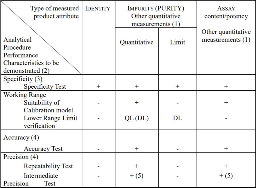
– signifies that this test is not normally evaluated
+ signifies that this test is normally evaluated
( ) signifies that this test is normally not evaluated, but in some complex cases recommended
Table (1) acquired from ICH Q2(R2)
The choice of performance characteristics used in Analytical Method Validation should be dependent on the method’s intended use. It is not always necessary to validate all analytical performance characteristics that are available for a specific technique.
RELATED ARTICLE: Method Validation vs Method Verification
For example, if the method is to be used for qualitative trace-level analysis, there is no need to test and validate the method’s Quantitation Limit or the linearity over the full dynamic range of the equipment since the main purpose of this method is to provide a successful detection/identification of the analyte.
For an efficient validation process, it is important to specify the right validation parameters and acceptance criteria. The more parameters, the more time it will take to validate. The more stringent the specifications or acceptance limits, the more often the equipment will have to be recalibrated and probably also requalified to meet higher specifications at any time. It is not always essential to validate every analytical performance characteristic, but it is necessary to define which ones are required.
Conclusion
Evaluating specific performance characteristics is crucial for ensuring the reliability of analytical procedures in the pharmaceutical industry. Parameters such as specificity, linearity, range, accuracy, precision, LD, LQ, and robustness collectively define the method’s capabilities and adherence to current GMP standards. The careful selection of these characteristics is vital for optimizing the use of analytical methods within the pharmaceutical industry framework.

